This blog post addresses the frequently asked queries about R Programming. After facing certain issues regarding R, I decided to tackle this situation in the best way possible. My thoughts were along the lines of creating an informative guide stating all the required information on R Programming.
Moving ahead with this approach, I have collected all the required data, arranged it in an easy-to-follow flow, which you can find further down this post.
Jump to Section
What Is R Programming?
R is a programming environment and software environment for data analytics, statistical analysis, graphics representation, predictive analysis, reporting, and research.
It is the most comprehensive statistical analysis package and standard statistical tests available for managing and manipulating data. It is an open-source programming language. R is a simple but well-developed language that supports the following:
- Data Processing,
- Statistical Analysis,
- Graphics,
- The rapid development of new tools that can be distributed as packages,
- Predictive Models,
- Machine Learning,
- Regression Model,
- Cluster Algorithm,
- Decision Tree Model.
When Should We Not use R Programming?
- When the data won’t fit into memory
- When run-time is crucial
However…
These are all areas of active development for R Programming and some partial solutions already exist.
Currently,
- R allows C, C++, and Fortran code to be called
- R supports multicore, grid, and GPU processing
- Some out-of-core algorithms exist (g. bigglm)
- Some types of very large structures (g. matrices) can be supported.
- Some key code has been rewritten in C/C++ (colSums, col Means)
- R can be called from a number of tools and it integrates into Hadoop (Big Data)
How to Work with R Programming?
Below is a step-by-step guide that can help you with working on R Programming:
- Ideally, you use Rstudio, an Integrated Development Environment (IDE). There are also plugins for Eclipse.
- If you work directly in R you can (should) write R commands into a text file (R script) and run it inside of R using the source() function. A good editor is Notepad++.
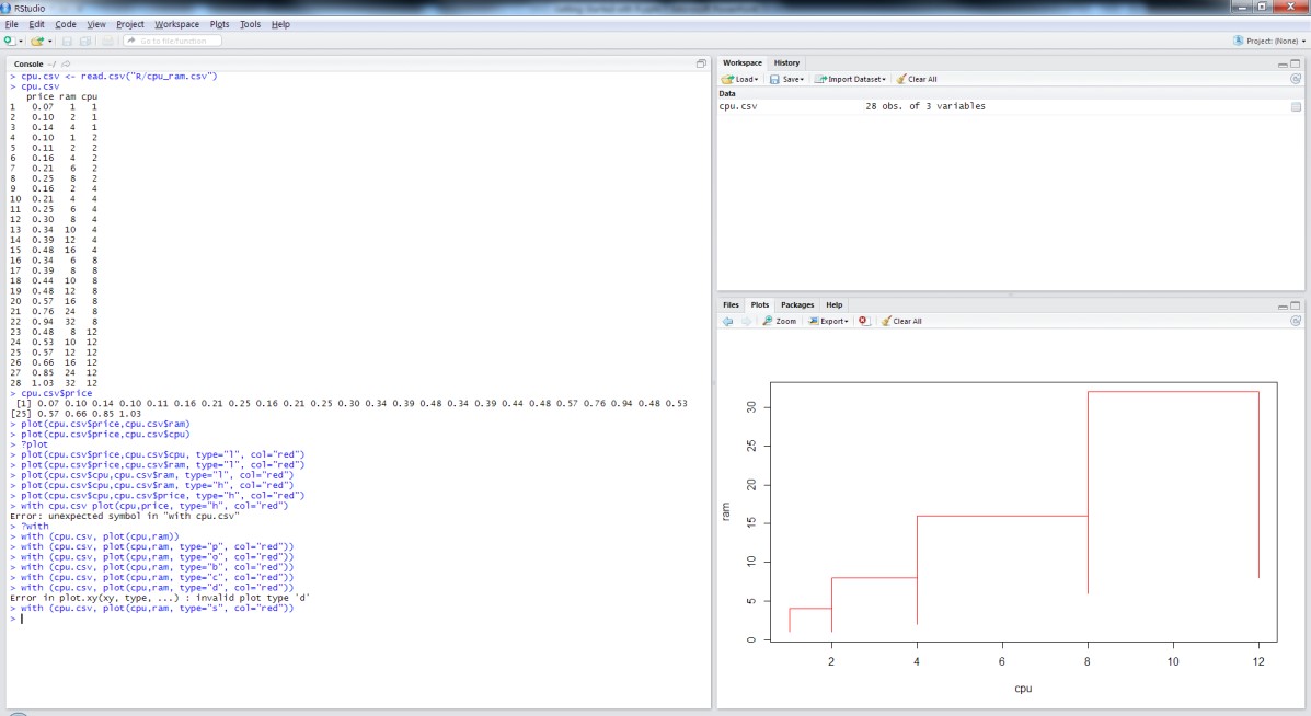
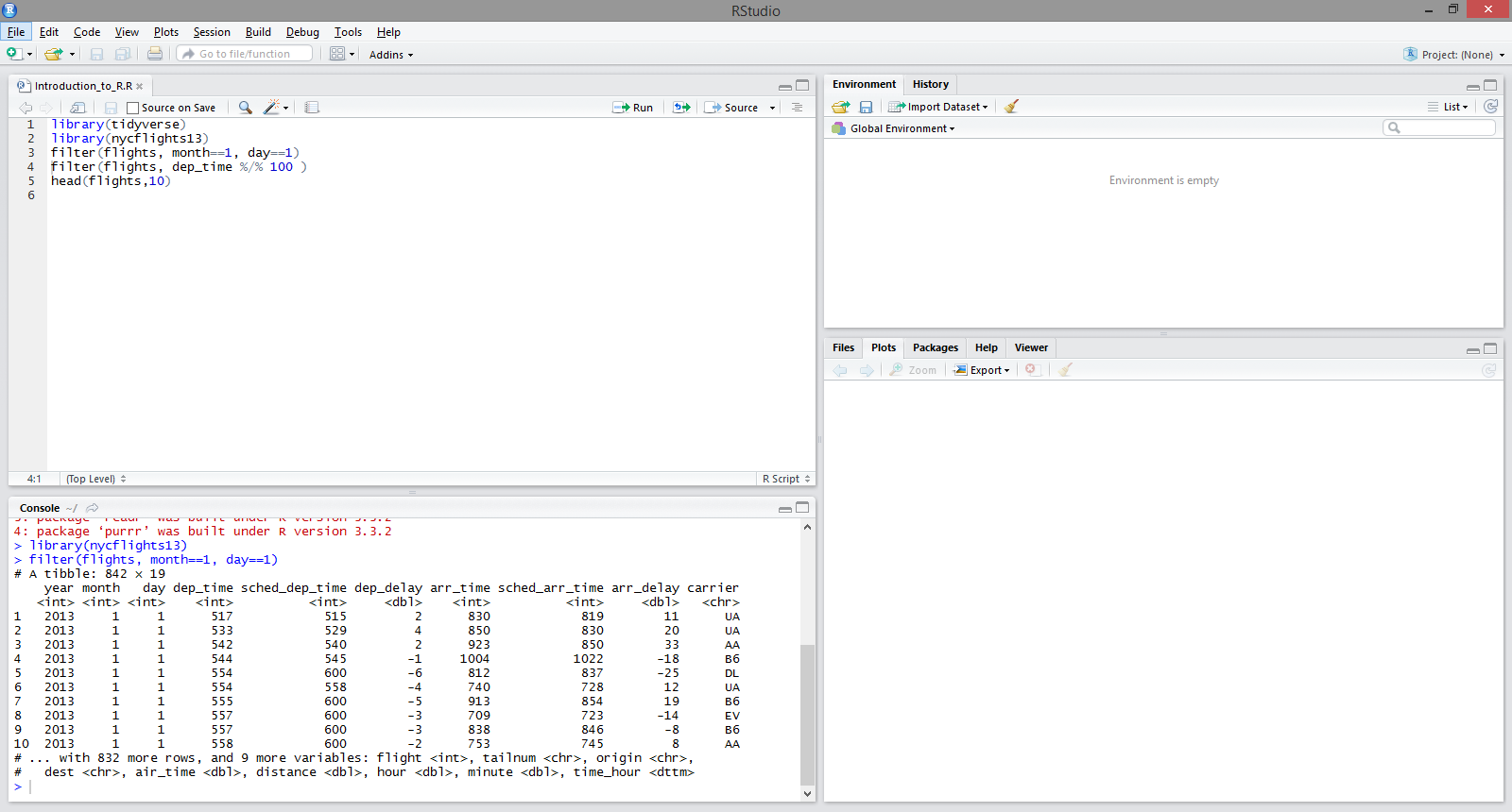
R Programming Studio
- Text editor to write an R script. CTRL+Enter or Run executes the current line or selection. It can automatically complete code with the tab key.
Source runs the whole script:
- List of objects in your R session (Environment) and list of executed commands (History).
Getting Help with R:
- R comes with an HTML help file that will be displayed in your browser
- help(anyfunction) or ?anyfunction use quotes for operators and special characters,
g. help (“%*%”) or ?”%*%” (%*% is the operator for matrix multiplication) - ??”any string” to search the R help file for any string (“” when the string contains blanks)
- Google is your best friend: use R as the first search term.
- com – for programming questions
- com – for statistics questions
- The R search engine http://www.rseek.org/
- R help mailing list at stat.ethz.ch/mailman/listinfo/r-help
- But only if you’re desperate!
- Google R style guide – how to write good R code
- http://google-styleguide.googlecode.com/svn/trunk/google-r-style.html
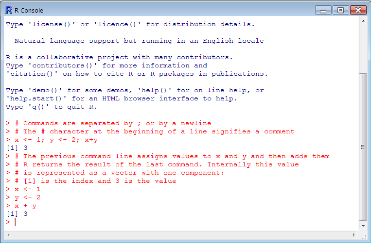
R Programming Console Window:
We can write commands in the input line text field and edit code almost like in a usual editor. But the R studio console window is better than from R console window. R console cannot complete the code by using the tab key. It shows the output in the next line not in other console windows.
R Objects and Values
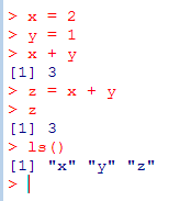
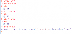
- R stores everything in objects;
- Values are assigned to and stored in objects using the <- or = operator;
- The operator <- can be used anywhere, whereas the operator = is only allowed at the top level (e.g., in the complete expression typed at the command prompt);
- You can write x <- y <- 5 and x = y <- 5, but not x <- y = 5 (<- has higher precedence);
- I will use = instead of <- for easier readability, but the Google R Style Guide says to use <-;
- A list of all objects in the current session can be obtained with ls().;
R is case sensitive, so A and a are different symbols and represent different objects
Basic Data Types
- character – string values, e.g. “abc”, “3.14”
- numeric – decimal values (real numbers), e.g. 3.14, -2.5
- integer – e.g. 1, 2, 3, -1456, …
- logical – TRUE or FALSE (you can use T or F instead,
but be careful because these are predefined variables
and can be changed by the user) - complex – a vector of complex numbers
Weird Values – Not Available, Non-existing, Impossible
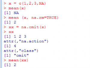
- The notion of a ‘missing value’ is as fundamental in statistics as the notion of zero is in arithmetic;
- The NA symbol allows R functions to do sensible things when missing values are encountered;
- Many R functions give you a choice of what to do when NAs are encountered: (na.omit=T, na.rm=T);
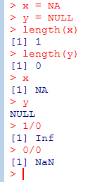
- There is a separate NULL symbol in R. NA is a value that exists but is unknown, whereas NULL indicates there is no value;
- A vector that contains just the value NA has length 1, whereas a vector that contains just the value NULL has length 0;
- NaN (not a number, Infinity).
Data Structures – Vectors: Vectors (as in computer science, not as in maths)
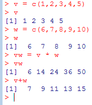
A set of contiguously stored values, which can be numeric or non-numeric. c() combines values into a vector or list.
(NB: There are no scalars in R, just vectors of length 1)
We can also use:
v = c(1,2,3,4,5) or v = c(1:5) results in the same vector v.
w = c(6,7:9,10) to obtain the same vector w
c(6,9:7,10) would result in (6,9,8,7,10)
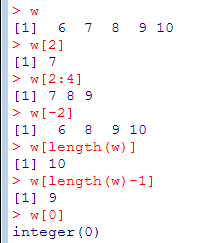
Access individual components of a vector by indexing them using square brackets. The first component has index 1. Index 0 reveals the type of components
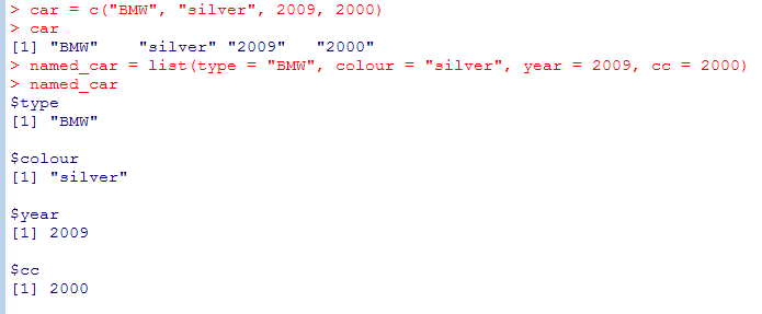
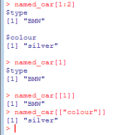
Data Structures – Lists. List are like vectors, but you can have elements of different types and you can insert or delete elements
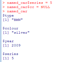
- List elements can have names and you can use them to retrieve values (list$colname)
[[ ]] extracts exactly one element without the label (different to [ ] which extracts a sublist and retains the labels). You can use computed values within [[ ]]
EX:
Data Structures – Factors
- Factors are variables that take on a limited number of different values
- They are often referred to as categorical variables.
- One of the most important uses of factors is in statistical modeling. Since categorical variables enter into statistical models differently to continuous variables, storing data as factors ensures that the modeling functions will treat such data correctly.
- R provides both ordered and unordered.
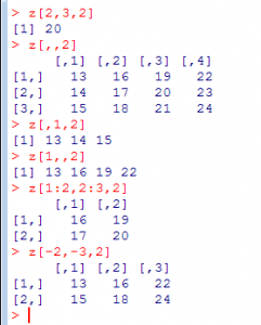
Data Structures – Arrays
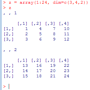
- Arrays: multi-dimensional (multiply subscripted) collection of data entries.
- Matrices (as in maths) – a 2-dimensional array.
- Turning a vector with 24 values into a 3 x 4 x 2 array
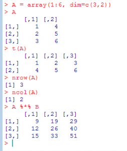
Data Structures – Matrices: Important special case of arrays with many operators and functions exclusively for matrices.
- t() transpose matrix
- nrow() number of rows
- ncol() number of cols
- %*% matrix multiplication
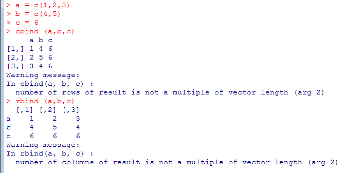
Column-wise (cbind) or row-wise (rbind) combination of vectors and matrices into matrices. Note the cyclical extension of vectors if they are too short for the function.
Data Structures – Data Frames
- A list with class “data.frame”. The components must be vectors (numeric, character, or logical), factors, numeric matrices, lists, or other data frames.
- Matrices, lists, and data frames provide as many variables to the new data frame as they have columns, elements, or variables, respectively.
- Numeric vectors, logicals, and factors are included as is, and by default, character vectors are coerced to be factors, whose levels are the unique values appearing in the vector.
- Vector structures appearing as variables of the data frame must all have the same length, and matrix structures must all have the same row size.
- Mostly, you will use it like a database table or spreadsheet.
- The simplest way to construct a data frame from scratch is to use the read.table() function to read an entire data frame from an external file.
- There is a simplified version of a data frame called a “tibble”. It tweaks some of the behavior to make life easier. To use them you need to install and load the package tibble (or tidyverse which includes packages like dplyr and tibble) – see http://had.co.nz/tibbles.html.
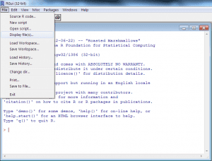
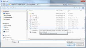
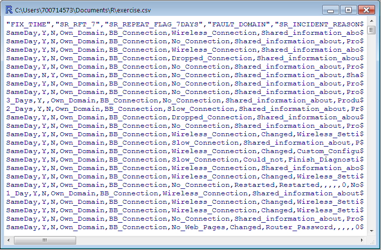
Use the GUI to view a data file in text format
(this does not load the data into R)
- If your data is in a CSV file, you can use read.csv() to read it into a data frame (a special case of read.table()). Use an expressive name for the object.
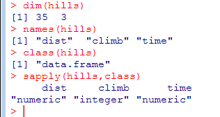
- dim() shows the dimensions (rows and columns), names() shows the column names, and sapply() is used here to apply the class() function to all columns of the data frame
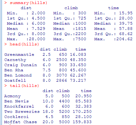
- summary() gives you a useful overview of your data frame
- head() shows the first 6 and tail() the last 6 rows. head(n=10) shows 10 rows etc.
Viewing and Editing Your Data Frame
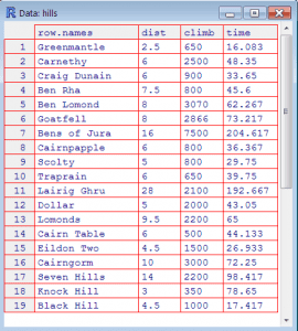
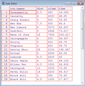
- View(): Show the data frame in a grid-like window. Notice it’s View, not view
- edit(): Invokes the editor. You must assign the result of the edit function to a data frame, e.g. data = edit(my.data)
Different Ways of Getting Data into R
- R supports several means of data entry
- Keyboard entry,
- Reading the clipboard buffer,
- Reading a delimited text file,
- Reading special file formats by using packages (e.g. EXCEL, SPSS, SAS),
- Pulling data from a URL by HTTP,
- Reading from a database that supports ODBC (includes Excel & MS Access),
- Reading from a database that supports JDBC,
- Reading an XML file,
- Reading a JSON file.
Reading Data from Files
- x = read.table(“C:\\temp\\my.data.txt”,sep=“\t”,header=T)
- Read text file my.data.txt in folder C:\temp, the values are separated by TAB characters, and the values in the first line are treated as column headers. Note that you have two write two backslashes instead of one in the path of a file.
- x = read.table(file.choose(),sep=“\t”,header=T)
- Brings up an Explorer window so you can click on the file you want
- x = read.csv(file.choose())
- A wrapper for read.table with sep=“,” and header=T
- x = read.table(“clipboard”,header=T)
- Reads the contents of the clipboard
- x = read.table(“http://fictitiousURL/datasets/my.data.dat”,header=T,sep=“\t”)
- Read a file from a URL
- Note: character columns are automatically converted into factors. If you don’t want this specify the option is = TRUE. (This is not necessary for tibbles, they don’t convert strings into factors)
- table is a wrapper for a more powerful function called scan(). If you have a file with a complex structure, that read.table can’t handle, use scan()
Using Data Frames
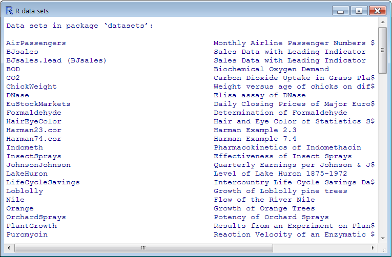
Let’s look at some of the sample data sets that come with R (run data() to see a list).
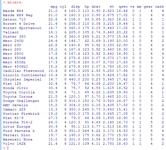
mtcars example data frame
(using built-in data frame mtcars)
- The columns of a data frame can be accessed by index or name
- mtcars[1] returns the first column as does mtcars[“mpg”].
- mtcars[1:3] returns the first three columns.
- If we use only one index it is assumed to be a columns index and we get all rows for the selected columns.
- We can also make this explicit: mtcars[ , 1:3] also returns all rows for the first three columns
- mtcars[1:5, ] returns the first 5 rows of all columns. Now we need to make clear that the index refers to columns and we need to write the comma to indicate that we want all columns.
- mtcars[1:5,1:3] returns the first 5 rows for the first 3 columns.
- mtcars[c(1:3,9:11)] returns columns 1-3 and 9-11.
- mtcars[c(“mpg”,”gear”)] returns the columns with the names mgp and gear.
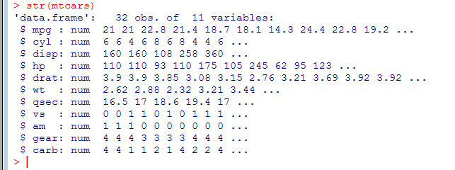
- str(mtcars) shows the structure of the data frame
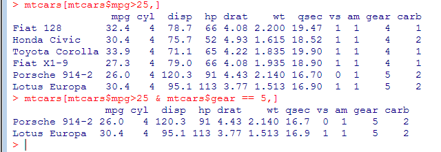
We can select rows that match only certain conditions (like a where clause in SQL). Note the comma indicating that we want all columns back.
- We can order a data frame by one or more columns. We can order increasing (default) or decreasing (similar to order by in SQL), but we can only specify one ‘decreasing’ option.
- Find all Mercs
- grep() uses regular expressions to search for matching strings.
- rownames() returns the name for each row of the data frame
(what actually happens is that R iterates over all rows of the data frame and checks if the name of the current row matches the condition, i.e. begins with ‘Merc’) - When we read data frame from a file read.table or read.csv will assume that there are row names if the second line has one more column than the first. By default, the first line is treated as a line of column names (unless we specify header=FALSE and then we cannot have row names either).
Using Data Frames – ‘Apply’ Functions
- sapply: apply one function to all columns of a data frame. The result is a vector.
- lapply: like sapply, but the result is a list
- tapply: apply one function to a vector grouped by the values of one or more factor (like a ‘group by’ in SQL).
Using Data Frames – ‘By’ Function
- by() is a wrapper for tapply() applied to data frames. The data frame is split by rows into subsets according to a factor and the given function is applied to all columns in each subset.
- The iris data frame has measurements of 150 specimens of 3 species of iris flowers. We want to calculate the column means for the first 4 columns grouped by the species.
- We can achieve the same results in different ways using by(), aggregate(), or sapply() which are all using slightly different arguments.
- Note: by() doesn’t work with mean you need to use colMeans (actually, applying mean to data frames is deprecated and you are supposed to use colMeans)
- We can select the first four columns from the iris data frame by iris[1:4], iris[ , 1:4] or by using column names iris[c(“Sepal.Length”, “Sepal.Width”, “Petal.Length”, “Petal.Width”)]
Apply and Replicate
- apply() is used for applying functions to the margins of matrices or arrays (‘sub-dimensions’).
- Replicate is a wrapper for the common used sapply for repeated evaluation of an expression.
- If we are interested in sums or means of rows and columns of a matrix M we can use the faster functions rowSums(M), colSums(M), rowMeans(M), colMeans(M)
Some Built-in Functions
- sum(), mean(), median, sd(), max() and min() calculate the sum, average, median, standard deviation, maximum and minimum.
Use the option na.rm=TRUE or na.rm=T to exclude missing values, otherwise the result will be NA if missing values (NA’s) are present in your data. - quantile() finds percentiles
- summary() gives the min, mean, median, max as well as the 25th and 75th percentiles
The dplyr Package
- The dplyr package by Hadley Wickham provides a number of useful “data wrangling” operations for data frames that are more intuitive to use than using square brackets [ ].
- All functions return a data frame (or tibble)
- filter (df, <expression>) selects all rows of the data frame df that match the logical expression.
- select (df, col1, col2, …) keeps only the named columns of the data frame df.
- summarise (df, name1=agg1(col1), name2 = agg2(col2), …) computes aggregations of data columns, like n() for count of rows, mean(), max(), etc. The result is a tibble.
- group_by(df, col1, col2, …) creates a data frame grouped by the named columns. You need to apply summarise() to the result to make use of it.
- arrange(df, col1, desc(col2), col3,…) lets you order your data by the named columns in ascending order (default) or descending order (if desc() is used)
dplyr: filter() example
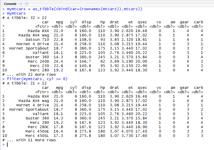
Create a tibble mymtcars from the built-in mtcars data frame by adding the row names of the original data frame as a new first column called “car”.
Printing the tibble mymtcars automatically only shows the first 10 rows and only as many columns as fit on the screen.
Using filter() to keep only rows with 6 or more cylinders.
dplyr: select() example:
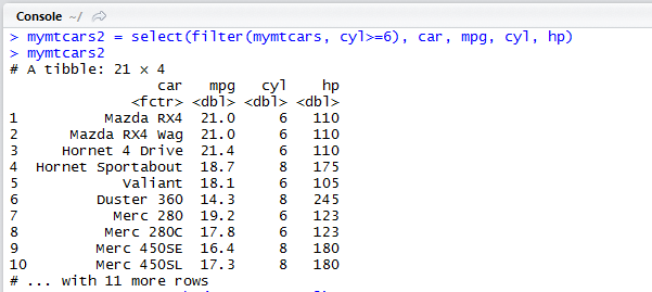
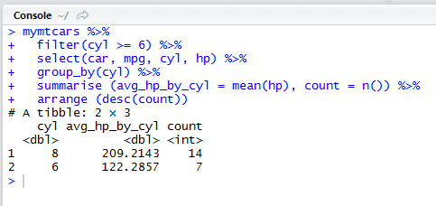
We keep only the columns car, mpg, cyl, and hp of the filtered data set.
dplyr: group_by() and summarise() example
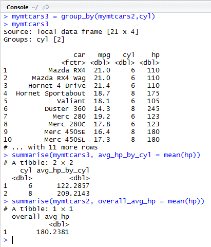
We group our tibble mymtcars2 by the number of cylinders (cyl) and save it in mymtcars3.
This creates a grouped local data frame. This is just a reference to the data with the grouping information added.
Then we summarise mymtcars3 for the hp column by using mean() as an aggregation function. This gives us a mean for each group of cylinder values.
If we use summarise on the ungrouped mymtcars2 instead, we get only one global average for hp.
Pipe operator %>% in dplyr package:
DPLYR provides a very useful operator. The pipe operator %>% (read as “then”)
Instead of creating intermediate result variables or nesting function calls we can use the pipe operator.
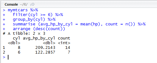
Here we compute a similar result to the previous 3 slides, but we are using the pipe operator. We take mymtcars, then we filter and keep only rows with 6 cylinders or more, then we group by cyl, then we use summarise to compute the average horsepowers and the count of rows per group and then we order the result by descending count of rows.
DPLYR vs SQL
On the right, there is an SQL query that produces the same result as the dplyr expression in R on the left.
- The dplyr filter expression appears in the SQL where clause
- The dplyr group_by is equivalent to the SQL group by clause.
- The dplyr summarise expression is represented by the aggregation functions avg() and count(*) in the SQL select clause.
- The dplyr arrange expression is equivalent to the SQL order by clause.
- Naming the mymtcars data frame is equivalent to the SQL from a clause that uses the table mtcars
Note that we don’t require a dplyr select here because the summarise automatically returns the columns mentioned in the group_by and computed within the summarise function.
In SQL we always have an explicit select to list the columns we want to see.
select cyl, avg(hp) as avg_hp_by_cyl, count(*) as count from mtcars where cyl >= 6 group by cyl order by count desc
Coercion – turn it into something it is not
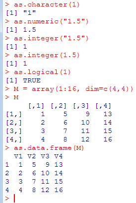
- R changes the type of an object (coercion) if the context requires it, but we can also do this explicitly using the ‘as.’ functions.
Basic Scatter Plot (base package)
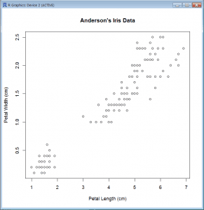
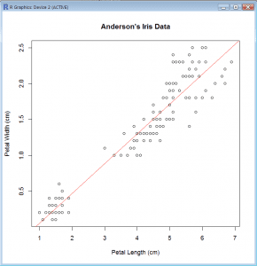
- plot(iris$Petal.Length, iris$Petal.Width, xlab=”Petal Length (cm)”, ylab=”Petal Width (cm)”,main=”Anderson’s Iris Data”)
- Plot() is a generic 2-dimensional x-y plot and plots y (iris$Petal.Width) over x (iris$Petal.Length)
- We can also use this syntax:
plot(Petal.Width~Petal.Length, xlab=”Petal Length (cm)”, ylab=”Petal Width (cm)”, main=”Anderson’s Iris Data”, data=iris) - The ~ operator signifies a formula in R.
y ~ x means that y is explained by x. - If the graphics command uses a formula, we use data= to specify the data frame and don’t need to use the $ notation.
Scatter Plot with Trend Line (base package)
- We can fit a regression line (line of best fit) using the function lm() which fits linear models.
- We fit a linear model and save it as a linear model object iris.lm
- lm = lm(Petal.Width~Petal.Length,data=iris)
- Then we use the abline() function to draw a straight line into the existing plot. It is very flexible and can draw pretty much any sort of straight line. Here it uses the linear model to draw the line. We also choose to plot the line in red.
- abline(iris.lm,col=”red”)
Scatter Plot with Factor
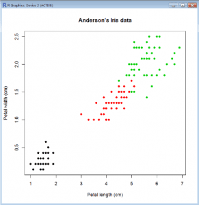
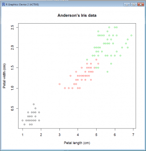
- plot(Petal.Width~Petal.Length, col=Species,xlab=”Petal length (cm)”,ylab=”Petal width (cm)”,main=”Anderson’s Iris data”, data=iris)
- Here we have used the categorical variable (factor) iris$Species to determine the color for each data point.
- This works because in R each color is associated with a number as is each level of a factor.
Scatter Plot with Factor
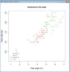
- We can also change the printing character for the symbols; pch = 16 produces dots instead of circles:
plot(Petal.Width~Petal.Length, col=Species, pch=16, xlab=”Petal length (cm)”, ylab=”Petal width (cm)”,
main=”Anderson’s Iris data”, data=iris) - If we want to use the factor to change the symbols, we can do that too, but we have to explicitly coerce it into numbers:
plot(Petal.Width~Petal.Length, col=Species, pch=as.numeric(Species), xlab=”Petal length (cm)”,ylab=”Petal width (cm)”, main=”Anderson’s Iris data”, data=iris)
Graphics Using the Singers Data Set
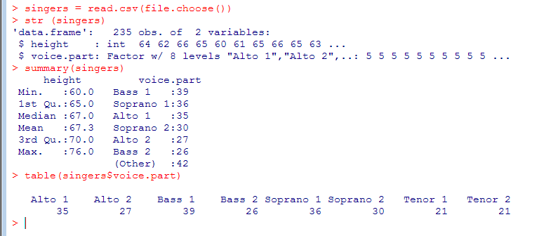
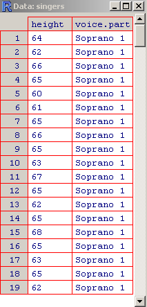
- Sample data set about the height of opera singers (in file singers.csv)
- We load the file via a file chooser. csv() assumes there is a header line by default
- table() provides a cross-tabulation (contingency table) that counts the combination of values given by the arguments, which have to be factors or lists
The Singers Data
- > View(singers)
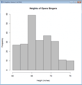
Histogram (Base)
- > hist(singer$height, col=”grey”, main=”Heights of Opera Singers”, xlab=”Height (inches)”)
- hist() produces a histogram
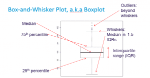
Box-and-Whisker Plot, a.k.a Boxplot
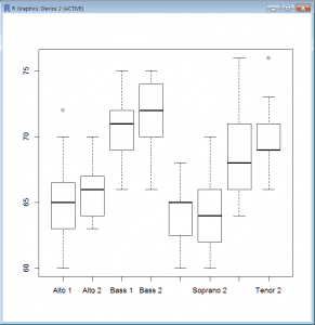
Boxplot (Base)
- = plot(singers$voice.part,singers$height)
- plot() is a generic x-y plot in R’s base package.
- Here, plot() produces a boxplot because voice.part is a factor.
- There is a dedicated boxplot() command with a slightly different syntax:
- = boxplot(height ~ voice.part, data=singers)
- The ~ operator signifies a formula in R.
y ~ x means that y is explained by x. - If the graphics command requires a formula, we use data= to specify the data frame and don’t need to use the $ notation.
The “lattice” Package:
- As well as base graphics R has the lattice package which attempts to improve on the basic graphics by providing better defaults and the ability to display multivariate relationships.
- In particular, it supports trellis graphs that display graphs conditioned on one or more other variables.
- There is much duplication between base and lattice, and some differences
- There are syntax differences between base and lattice, such as the way legends are produced
- lattice allows all charts to be trellised
- lattice does not contain pie charts!
- The typical format is graph_type(formula, data=) where graph_type is selected from the listed below.
- formula specifies the variable(s) to display and any conditioning variables.
- For example ~x|A means display numeric variable x for each level of factor A.
- y~x | A*B means to display the relationship between numeric variables y and x separately for every combination of factor A and B levels.
- ~x means display numeric variable x alone.
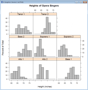
Trellis of histograms (lattice)
- library(lattice)
- histogram(~height|voice.part, data=singers, col=”grey”, main=”Heights of Opera Singers”, xlab=”Height (inches)”)
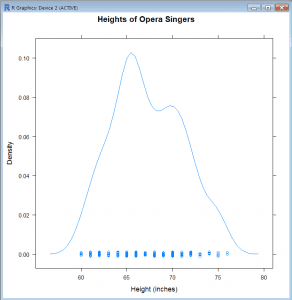
Density Plot (lattice)
- densityplot(~height, data=singers, main=”Heights of Opera Singers”, xlab=”Height (inches)”)
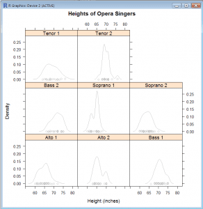
Density Plot: Show Distribution of Height within Voice Part
- densityplot(~height|voice.part, data=singers, col=”grey”, main=”Heights of Opera Singers”, xlab=”Height (inches)”)
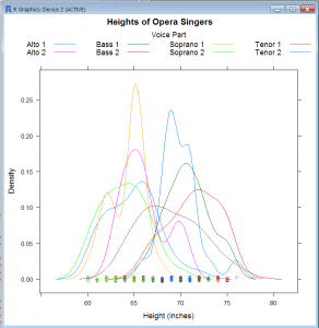
Density Plot: Overlaid Plot with Legend
- densityplot(~height, groups=voice.part, data=singers, main=”Heights of Opera Singers”, xlab=”Height(inches)”, key=list(space=”top”, columns = 4, title=”Voice Part”, cex.title=1))
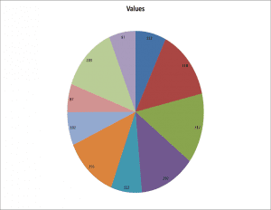
Pie Charts (Excel) versus Dot Charts in R
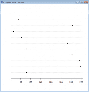
Value = c(112,218,217,202,113,193,102,87,203,97)
Pie Charts (Excel) versus Dot Charts in R
- We cut&paste the data from Excel into R using the read.table() function
data = read.table(“clipboard”,header=T) - Then we produce a Dot Chart using pch=16 to obtain filled in dots instead of the default printing character (circle).
dotchart(dch.data$Values,pch=16) - The dot chart shows clearly that we have two groups of values.
If you want to get the chart out of R
- In RStudio use the export button of the Plot window.
- The Windows Snipping Tool in Accessories allows you to copy anything off the screen and save it as a PNG or JPEG
- ALT-PrtScn copies the active window to the clipboard. From there you can paste it into any Microsoft Office application or paste it into Microsoft Paint (in Accessories), crop it, and save it as a PNG, or cut & paste it further.
- R can save your chart as a PNG, BMP, PDF, JPEG, or TIFF picture
- Look at help (png), help (bmp), etc. for syntax.
# Divert a plot to a png file
png(“myplotfile.png”) # You can use file.choose() here if you want
Summary
Following points can be put up a summary of the whole article:
- R is well-equipped with data manipulation tools for all sorts of purposes.
- Ideal for data manipulation as well as statistical analysis.
- R Package is a collection of R programming functions with comprehensive documents.
- R has a wider selection of graphics, and these are much better chosen, than those available in Excel.
- One of the early benefits of learning R, even if you don’t want, need or understand the advanced statistical tools, is being able to use this wider range of graphical displays.
- We have only touched the surface of what can be done with R but hopefully, you will now be able to do some basic data manipulation and generate some useful graphics by yourself.
- To learn more, make use of the internal help function (help(…) or ?…) and have a look at the references on the next slide.
- COVID-19: How We Are Dealing With It as a Company - March 23, 2020
- Agile Testing – The Only Way to Develop Quality Software - February 8, 2019
- How to Perform System Testing Using Various Types Techniques - May 16, 2018



![Select the first four columns from the iris data frame by iris[1:4], iris[ , 1:4] or by using column names iris[c("Sepal.Length", "Sepal.Width", "Petal.Length", "Petal.Width")] Select the first four columns from the iris data frame by iris[1:4], iris[ , 1:4] or by using column names iris[c("Sepal.Length", "Sepal.Width", "Petal.Length", "Petal.Width")]](https://www.loginworks.com/wp-content/uploads/2017/12/r36-1.png)

This blog is really amazing, any unknown will definitely get something good on R Programming….Good Job Prashant…I really admire your Hardwork….:-)
Really amazing..anyone can easily get the basic of R programming.